Michael Beeson's Home Page

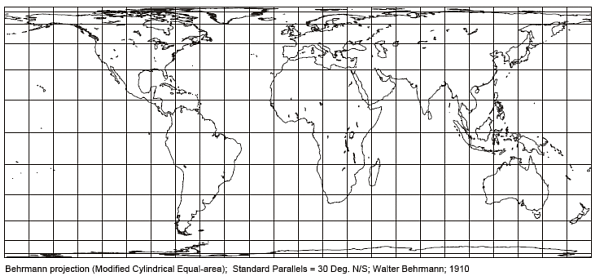
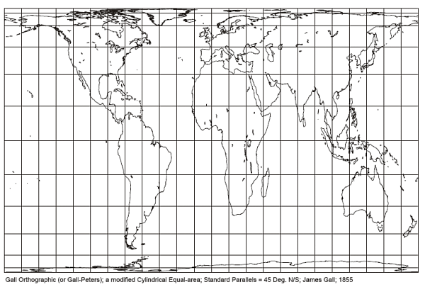
Projections used in mapmaking

The problem of representing a portion of the spherical earth on a flat map is fundamental to the mapmaker's craft. That is accomplished by means of a projection, which is a correspondence between part of a sphere and part of a plane.

We may list the following desirable features of a map:

Unfortunately it is mathematically impossible to achieve the first two of these aims simultaneously, let alone all three of them. That is why there are several hundred projections that have been used in cartography. Here we will survey a few of them.

Mathematically, it is easier to consider the map from the plane to the sphere than from the sphere to the plane. The mathematical property corresponding to the preservation of small shapes is conformality.

Equal area cylindrical projection. (Lambert cylindric projection) In this projection, the sphere is projected onto a cylinder tangent to the sphere at the equator. Each point is projected onto a point on the cylinder that is the same height above the equatorial plane as the point being projected. The cylinder is then unrolled to make a planar map. This projection is not actually useful for maps, but we consider it just to point that out.

Projection onto a secant cylinder. Here, the cylinder cuts the sphere on two parallels, of equal but opposite latitudes, for example, 45 degrees north and south. Each point is projected onto a point on the cylinder that is the same height above the equatorial plane as the point being projected. Another way of thinking of these projections is that they are just the Lambert cylindric projection, but then the after unrolling the cylinder, a horizontal compression is applied. The compression factor determines the "standard parallel" where the scale is the same on the map and the globe, i.e. the parallels where the compressed cylinder intersects the sphere. Several of these projections, differing only by the standard parallel, have names:

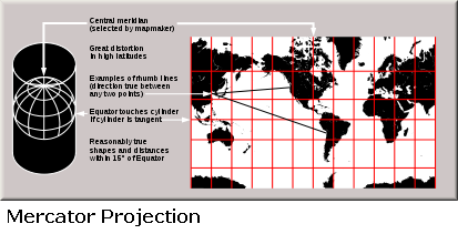
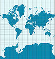
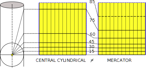
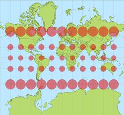
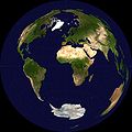
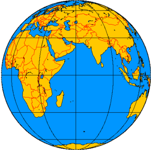
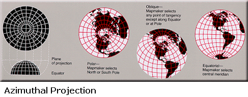
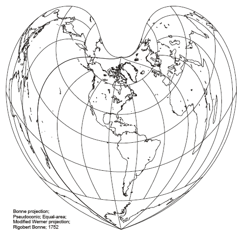
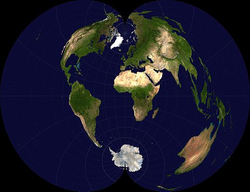
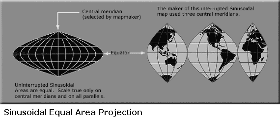
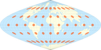
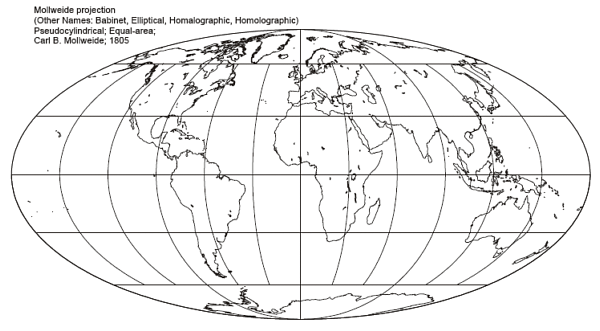
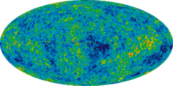
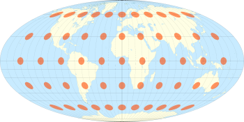
Projection from the center onto a tangent cylinder. Again, the cylinder is unrolled to make a planar map.

Mercator projection. In this projection, the meridians (lines of constant longitude) are vertical lines, and the parallels (lines of constant latitude) are horizontal lines. The meridians are equally spaced, and the spacing of the parallels is computed to make the map conformal. Here's another image of a Mercator map, and here's a comparison of the Mercator projection to the Lambert cylindrical projection. Mathematical formulas can be found here. Tissot's index of distortion can be seen here. My photos of Mercator's 1569 map in the Rotterdam museum can be seen here.

Stereographic, or azimuthal, projection. In this projection, the plane of the map is the plane of the equator of the earth, and each point P on the sphere is connected to the north pole by a line. Where that line meets the plane of the map is the projection of P. It is also possible to use an arbitrary point of the sphere, instead of the north pole, as the point of projection.

Central, or gnomic, projection. Here the plane of the map is a tangent plane to the sphere, and the image of a point P is found by drawing a line from the center of the earth through P. The image is the point where this line meets the plane of the map. This is the earliest projection: it was used by Thales in the 6th century BCE to construct the first world map.

Lambert azimuthal equal-area projection. Here the images of the meridians are radial lines, as in the azimuthal or gnomic projections, and the images of the parallels are concentric circles; but the radii of those concentric circles are adjusted to give the map the equal-area property. Namely, the radius of the circle corresponding to a given parallel is the chord distance of that parallel from the pole. In this image you can see the geometry of the projection. Mathematical formulas are here.

Orthographic polar projection. A hemisphere can be mapped onto a plane by simply taking a photograph of it. If the north pole is the center, the meridians will be radial lines, and the parallels will be concentric circles, whose radii are (proportional to) their actual radii on the sphere. This projection is the one usually chosen for maps of the moon, since it corresponds to how we see the moon from Earth. The center does not have to be the north pole; the linked image has its center elsewhere. Mathematical formulas can be found here.

Azimuthal equidistant projection. The meridians are radial lines, and the parallels are concentric circles, but this time their radii are chosen to be proportional to the difference in latitude between the parallel and the north pole, i.e., 90 degrees minus the latitude. In other words, one degree of latitude always increases distance from the center of the map by the same amount.

The above projections either project the sphere directly onto a plane, or they project it onto a cylinder that can then be unrolled into a plane. It is also possible to project the sphere onto a cone, which can then be unrolled into a (piece of) a plane. We can either use a cone tangent to the sphere, or a secant cone that passes through two circles of latitude. To determine such a projection, we make the following choices: First we select either a circle of latitude for the tangent projection, for example thirty degrees, or we select two circles of latitude for the secant cone. (That first choice determines the tip of the cone.) Then we choose a point on the sphere's north-south axis to serve as the center of the projection. This might be the center of the sphere, but it could also be some other point.

Bonne equal-area projection. In order to map a certain region, for example the United States, we pick a central meridian and a central parallel. We use a tangent cone at that parallel to determine the image of the central parallel (which will be a piece of a circle); that tangent cone also determines where the meridians will cross the central parallel. The image of the central meridian is a vertical line perpendicular to the image of the central parallel. Then the images of the other parallels are concentric circles, whose radii are determined by requiring the scale along the central meridian to be the same as the scale on the central parallel. Finally, the images of the other meridians are determined by the requirement that they be perpendicular to all the parallels.

Albers equal-area projection. This is the projection onto a secant cone. There are two standard parallels (where the cone intersects the globe). Mathematical formulas can be found here.

Polyconic projection. As Deetz and Adams describe it, in this projection "The central meridian is represented by a straight line, and the parallels are represented by arcs of circles that are not concentric, but the centers of which lie in the extension of the central meridian. The distances between the parallels along the central meridian are made proportional to the true distances between the parallels on the earth. The radius for each parallel is determined by an element of the cone tangent along the given parallel. When the parallels are constructed in this way, the arcs along the circles representing the parallels are laid off proportional to the true lengths along the respective parallels." The name polyconic arises from the fact that many cones are used, one cone for each parallel. Mathematical formulas can be found here.

Finally we have the class of pseudo-cylindrical projections. In these projections, each parallel is represented as a horizontal line, and a selected central meridian is represented as a vertical line. The scale is true along each parallel, i.e. the distance between two points on the same parallel is the same as on the globe. Once we determine the spacing of the (images of the) parallels, this condition will determine the images of the meridians, which will then curve towards the center of the map as we move to the north. It is the rule for determining the spacing of the parallels that determines the name of the projection:

Sinusoidal projection. The parallels are so spaced that the distance between parallels on the map is the same as the distance between parallels on the globe. The name comes from the fact that, on the map as on the globe, the length of each parallel is proportional to the sine of the latitude, so the outline of the map is composed of two sine curves. Because this projection induces a large distortion of shapes, one also has a split sinusoidal projection, made from (for example) three sinusoidal projections on different central meridians. Shapes will be more accurate, but then you have the map split into three parts. The simple mathematical formula is here. Although this projection induces distortion of large shapes, the local distortion is small, as you can see in this plot of Tissot's index of distortion.

Mollweide projection. The spacing of the parallels is determined by the condition that the area between any parallel and the equator on the map is proportional to the area between that parallel and the equator on the globe. Of course that will then be true also for the area between two parallels. Mathematical formulas are here. This projection has been used to present the map of the cosmic background radiation (projections can be applied to the cosmic sphere as well as the terrestrial sphere). Here you can the local distortion of this projection. This projection is not often used for maps, probably because it distorts the shapes of continents so much, even though its local distortion is small. But for a cosmic-radiation map, that doesn't matter, since we have no expectation about the large-scale shape.

For more information see my sources:

Summary of map projections by Peter H. Dana of the Geography Department of the University of Texas.

Radical Cartography

John P. Snyder, Flattening the Earth: Two Thousand Years of Map Projections, 1993, pp. 112–113, ISBN 0-226-76747-7.

Deetz, Charles, and Adams, Oscar, Elements of Map Projection, with Applications to Map and Chart Construction, U.S. Coast and Geodetic Survey, 1934. Deetz was senior cartographer and Adams was senior mathematician . Luckily it is now free of copyright, so you can read or download it right here if you want. But it's a 28 megabyte file so it might take a few minutes.

There are Wikipedia articles and MathWorld articles on many of the individual projections listed above.